


Aug07
Visualizing Data with ggridges: Techniques to Eliminate Density Plot Overlaps in ggplot2
When it comes to visualizing data with a histogram and dealing with multiple groups, it can be quite challenging. I have recently come across a ...
Mar15
DuckDB Local UI is Awesome!
Discover how DuckDB Local UI revolutionises your data exploration experience. After years of using external tools, DuckDB’s native interface provides a seamless, quick, and intuitive ...
Jan05
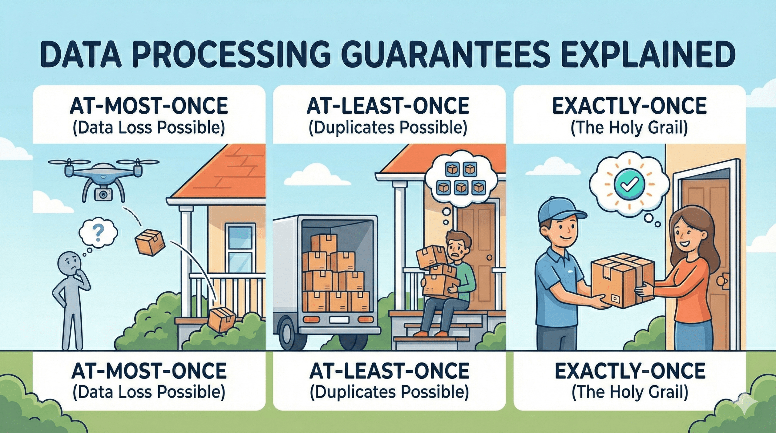
Data Processing Guarantees Explained: Exactly-Once, At-Least-Once, and At-Most-Once
Learn the difference between data processing guarantees (At-Most-Once, At-Least-Once, Exactly-Once) with simple real-world examples. Perfect for data engineering beginners